Note: this is an old post, beware.

Quick introduction

In this post I will show the process and details of developing TMTrackNN — a track generator for TrackMania.

A while ago when I started learning about Machine Learning, I wanted my first project to be something that is not a toy problem, nor something that is already extra common (e.g image classification). Therefore I started looking into generating tracks for my favourite racing game — TrackMania.

TrackMania is a racing game in which the goal is to drive the fastest time on a given track / map. Apart from the campaign tracks, you can build your own tracks in the map editor.

The tracks can vary greatly from their style, difficulty and length. Most competitive tracks involve maintaining good flow throughout the track itself. There are many track “styles” — one of the most popular style is tech — it features tight turns and many drifts.

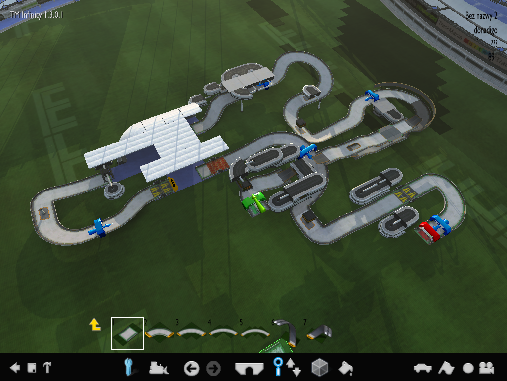
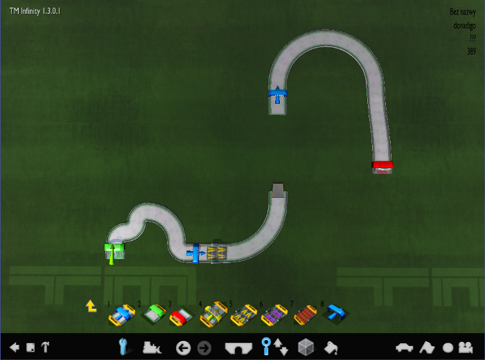
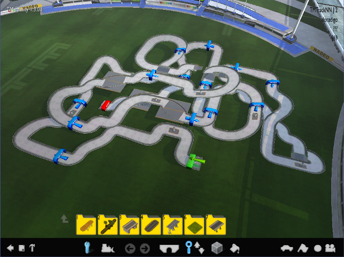
Here’s an example of such track built in a map editor:

What is the data?

Before going into details, let’s look at what makes up a TrackMania map.

A map is made up of series of blocks, placed on an available area of 32x32x32 units.

Each block has it’s three main properties:

• Block name
• Position
• Rotation

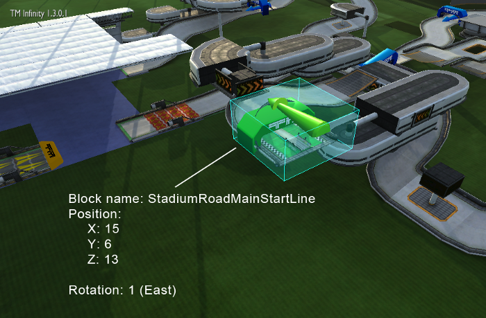
The block name represents the block type — if it’s a start block, a turn, a finish block etc. There are ~300 of those block types in the Stadium environment.

Position is straightforward — it’s made up of the X, Y, Z coordinates based on where the block is on the map.

Rotation is a digit between 0–3 which represents what direction the block faces:

• 0 - north
• 1 - east
• 2 - south
• 3 - west

All of this data can be pulled from a .Gbx file that TrackMania saves when saving the track. After writing the entire parser for those .Gbx files to pull this information I went ahead and started getting actual data — the tracks.

Getting the data and preprocessing

This step is sometimes very hard to overcome or can even be expensive for ML projects.

In this case the process was relatively easy. Conveniently there’s already a website called Trackmania Exchange (TMX) which provides a large collection of tracks made by people. The tracks can be sorted by their style and award count. I quickly wrote a Chrome extension to download all tracks on the current page and downloaded ~3500 1-minute tech tracks. On average a track has around 100 blocks after preprocessing.

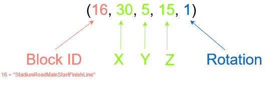
Preprocessing involves reading the map file and extracting the blocks from it. preprocessing.py does that using gbx.py, then processes this information and saves a simplified structure of each track. Here’s an example of one entry in the training data file:

('1170108.Replay.Gbx’, [(16, 30, 5, 15, 1), (282, 30, 4, 15, 3), (6, 31, 5, 15, 1), (282, 31, 4, 15, 0), (6, 29, 5, 15, 2), (282, 29, 4, 15, 1), (6, 29, 5, 14, 3), (282, 29, 4, 14, 1), (6, 30, 5, 14, 1), (67, 30, 4, 12, 2), (265, 29, 5, 13, 1), …)

The first element of the tuple is the filename of the replay. The second is a list of tuples, each representing one block on a map.

Visualizing the data and getting… stuck

We’ve collected the data, preprocessed it to a simple data structure, it’s now time to visualize the data. Because the track is a sequence of blocks we will need something simple that will show how the sequences look like. visualization_pygame.py does exactly that.

Looking at it we have our first problem that actually took the most time for me to overcome. The data is chaotic. The sequence doesn’t represent the actual path the track is meant to be driven which is how we would like to have the data look like.

The first block in the sequence should be the green start block on the left, then the yellow boosters etc. but that is not the case here. Eventually in the future we would like to feed this data into a RNN e.g an LSTM and generate tracks one block at a time. A lot of blocks are placed randomly, without any structure because of how the game saves the map — the block list is saved in order of how the player placed them. So if someone built a large chunk of track and then decided to go back and “fix” some part of the track, which is quite common — this is how the data will look like.

I thought about this for a long time and made many experiments along the way — from applying a Depth First Search to trying to sort the blocks by hand — which obviously was a crazy idea — one which would take too much time.

Instead I came up with a much better idea — to pull this information from already available replays.

Going back

Because replays are saved in the same file format, but are new information that my parser didn’t handle — I had to add support to parse replay files which surprisingly wasn’t that difficult and… download new data.

Now, instead of downloading raw map files, I downloaded replay files which also happen to contain the map that the replay was recorded on. Once again, this also meant that I also needed to add some code to take the replay data and trace all the blocks. I preprocessed them again and… success!

More data?

At this point our data starts to make sense, the sequences are in the order, and are saved in a simple format. One way to get more data… is either by scraping more data, or using data augmentation — which is often applied in image classification to improve model’s performance.

The track itself cannot be moved (will have no effect on the training data later) or “scaled” but instead we can randomly rotate all the blocks with respect to the map.

So for example, this track:

becomes:

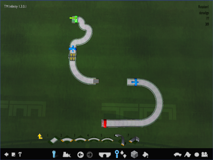
This makes our dataset size 4x larger as there are in total four cardinal rotations possible.

Model architecture

To be able to generate new tracks, we need to be able to sample from possible continuations of a track. At the moment TMTrackNN uses two neural networks, one for predicting the next block given a sequence of blocks, the second predicting it’s position in the map.

The block model receives a sequence of previous block placements. Each previous placement contains a one-hot encoded block type. At the output the network simply predicts the block type to put next. The output’s loss function is the softmax function.

The position model receives a complete sequence information about previous block placements. The model is fed with an encoding of previous blocks. Each encoding consists of a one-hot encoded block type, normalized a X, Y, Z vector from previous block and finally a one-hot encoding of it’s rotation.

Since we want to predict the next block in the sequence we ask the block model to predict the next block type. Then we ask the position model to predict the position of that block type by encoding it as a last time step in the sequence that is fed to the position model. Therefore the last block in the sequence consists only of the one-hot encoding of the block type and position and rotation vectors are filled with -1’s.

The position model’s output is two features: the vector to add to the position of last block to get a new position of the new block and the rotation of the new block. Their loss function is mean squared error and softmax respectively.

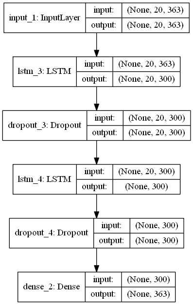
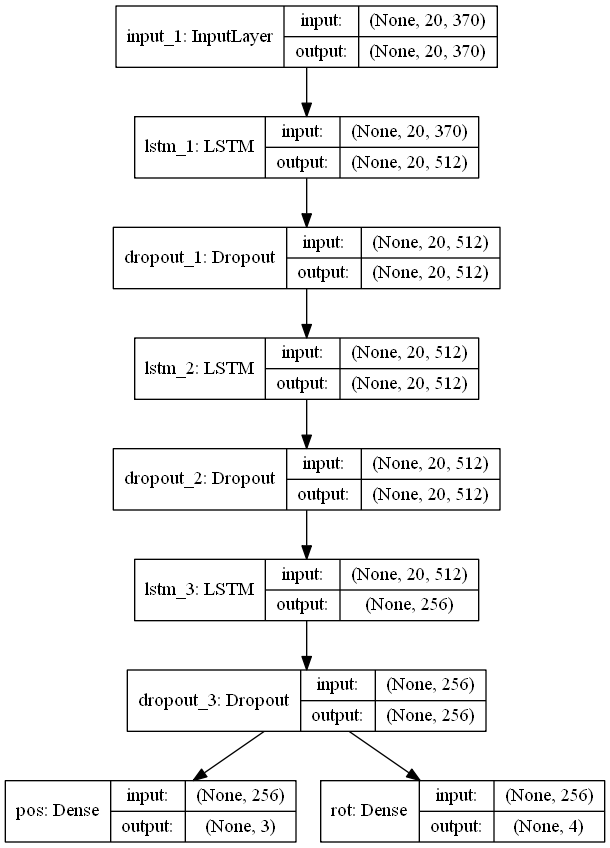
Models are currently implemented in Keras and here are their architectures:

• Block model
  

• Position model
  

Preparing data for training (code)

To be able to feed the data to our models we need to normalize it and transform the block tuples we’ve seen before to vectors.

For encoding a tuple, we will encode each feature separately, concatenate them all and feed it to the network. We will one-hot encode the block ID so that 14 becomes:

[0, 0, 0, 0, 0, 0, 0, 0, 0, 0, 0, 0, 0, 1, 0, 0, 0, 0, 0, 0, 0, 0, 0, 0, 0, 0, 0, …]

Before encoding position, we will transform to a vector that represents it’s position relative to the last block so that this block sequence:

[(14, 15, 5, 15, 0), (6, 14, 5, 16, 0)]

becomes this:

[(14, 0, 0, 0, 0), (6, -1, 0, 1, 0)]

because:

[14, 5, 16] — [15, 5, 15] = [-1, 0, 1]

The reason for doing this is that with this transformation we don’t need to care about the map size anymore, and we’re not restricting our inputs to be always a maximum of 32x32x32.

We will scale all those vectors with MinMaxScaler from sklearn to make sure that they stay in the range of [0, 1].

Finally, the rotation can be easily one-hot encoded also, so that rotation 0 (north) becomes:

[1, 0, 0, 0]

We concatenate all of those arrays and e.g our final encoding of block (6, -1, 0, 1, 0) is:

[0, 0, 0, 0, 0, 1, 0, 0, 0, 0, …, 0.47, 0.55, 0.63, 1, 0, 0, 0]

For splitting sequences I’ve used the sliding window method with lookback of 20 which means each block in a sequence will have a sequence of it’s 20 previous blocks as the input. I also used 0-padding for sequences that are shorter than the mentioned 20.

The final input for one sample for the position model looks like this:

[0, 0, 0, 0, 0, 0, 0, 0, 1, 0, …, 0.39, 0.75, 0.13, 0, 0, 1, 0]

[0, 1, 0, 0, 0, 0, 0, 0, 0, 0, …, 0.45, 0.55, 0.24, 0, 0, 0, 1]

[0, 0, 0, 0, 0, 0, 0, 0, 1, 0, …, 0.09, 0.60, 0.38, 0, 1, 0, 0]
...

For the block model, we only need the first encoding of the block ID, since it only predicts what block type would likely to be put next.

Generating new tracks (code)

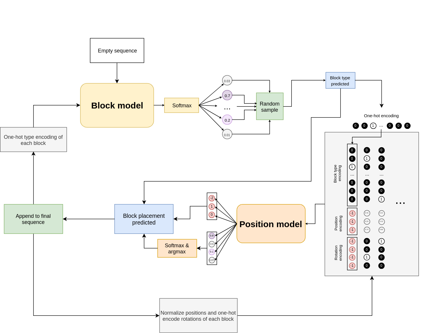
When generating a new track, we begin by randomly placing a start block on the map. We encode this sequence of length 1 and feed it to the block model. At the output we get probabilities of the block type to put next. We apply a temperature to this output, and then sample.

After that, we encode the inputs again but for the position network, run them through the network and receive real-valued position vector and a rotation probability vector.

After that, we perform a bunch of additional checks (if the track doesn’t exceed map size etc.) in the code to make sure that the output is somewhat correct (after all, the networks aren’t always perfect) and repeat the process again until we reach the desired track length in blocks.

At the end of the track we need to put a finish block so that we can actually finish it. This is done by omitting the whole “block prediction” step in the graph down below and just asking the position network to predict the position for a finish block:

Finally, we translate all the position vectors to actual map coordinates so that the track can be saved for the game to read.

Results

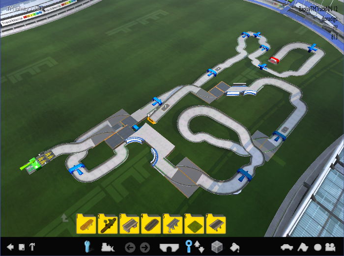
After training the networks and going through many more problems that I faced, generated tracks are often drivable by a human and resemble the “tech” style. Here are a couple of screenshots of some generated tracks:

Conclusion

I’m sure there is a ton room for improvement (data cleaning, better models, hyperparameter tuning to only name a few). This is my first ML project and I learned a lot about many things. Overall I’m really happy for how it turned out.

I skipped some of the details in this post to keep it not a too-long read, but I hope it was at least an interesting read for you.

Check out the project on GitHub and if by any chance you’re a TrackMania player, check out the release page for downloads or some tracks that were generated with TMTrackNN.

Thanks for reading!